Simulating the OLS Consistency When X and ε are Dependent

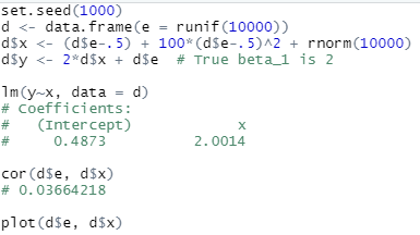
This morning I saw an interesting tweet by Nick HK, who ran a simulation to convince himself of the fact that OLS consistency only requires Corr(X, ε) = 0 but not independence:

I still find it hard to believe that OLS consistency only relies on X being uncorrelated with ε, not independent of ε, and I occasionally run a simulation to re-convince myself.

I had no doubt about the conclusion, primarily because I had kindly returned most of the things I learned in the linear models class to the instructor after I passed the exams more than a decade ago (sorry, Dr. Nettleton!).

What I found not quite convincing was that Nick only ran the simulation once. A single estimate of $\beta$ is not convincing to me to show that the OLS estimator is consistent, even if its value (2.0014) is fairly close to the true parameter (2).

BTW, this is off-topic, but usually I’m slightly less convinced about simulation results obtained from a fixed random seed. Fixing the seed is common practice for reproducibility, but reproducibility should be independent with the seed (for random simulations, I think reproducibility “in the ballpark” is more useful than “digit-to-digit” reproducibility).

A silly counterexample

If we could conclude consistency from an estimate in one simulation, we would conclude the same thing by estimating $\beta$ from the equation y = 2 * x + e, where e = 0.0014 * x, which means ε and X are perfectly correlated:

x = runif(10000)
e = .0014 * x
y = 2 * x + e  # i.e., y = 2.0014x
lm(y ~ x)

Apparently it would not be sensible, even if we get the same estimated value (2.0014), to conclude that consistency still exists when Corr(X, ε) = 1.

N needs to increase to illustrate consistency

If I remember correctly, consistency means convergence (of $\hat{\beta}$ to $\beta$) in probability, as the sample size N increases to infinity. That means we need to examine the behavior of the estimator as N increases. Below is a function to estimate the slope of the simple linear regression, with a slight modification (changing lm() to lm.fit() for speed) based on Nick’s R code:

beta_est = function(N = 10) {
  e = runif(N)
  x = (e - .5) + 100 * (e - .5)^2 + rnorm(N)
  y = 2 * x + e
  res = lm.fit(cbind(1, x), y)
  res$coefficients[2]  # the slope
}

Next we estimate the coefficient 30 times for different sample sizes N = 10, 210, 410, ….

Ns = rep(seq(10, 15000, 200), each = 30)
bs = numeric(length(Ns))
for (i in seq_along(Ns)) {
  bs[i] = beta_est(Ns[i])
}

Last we draw a scatterplot to illustrate how the estimate “converges” to its true value. Note that is is only an illustration of the overall trend. Of course, an illustration is not a proof.

par(mar = c(4, 4.5, .2, .2))
plot(
  Ns, bs, cex = .6, col = 'gray',
  xlab = 'N', ylab = expression(hat(beta))
)
abline(h = 2, lwd = 2)
points(10000, 2.0014, col = 'red', cex = 2, lwd = 2)
arrows(10000, 2.0014, 8000, 1.99)
text(8000, 1.987, 'Estimate from the simulation
 mentioned in the tweet')

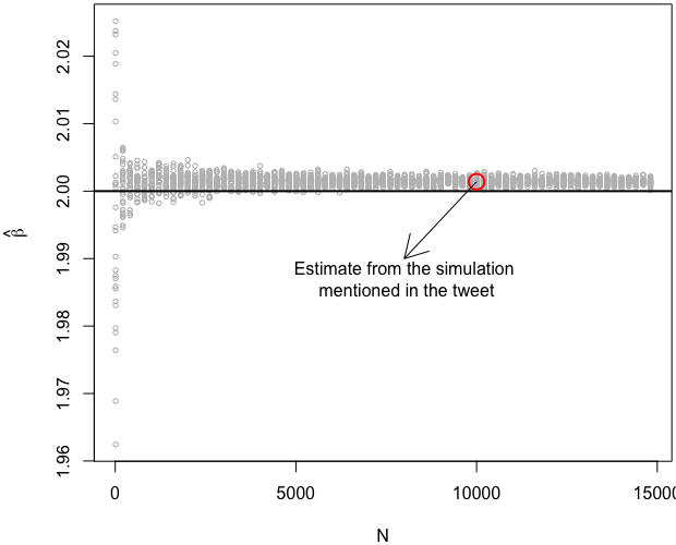
I have also marked the value 2.0014 in the plot corresponding to the sample size 10,000.

Does it really converge to the true parameter value?

At the first glance, the estimator appears to be converging indeed. However, after I marked the true parameter value (again, 2) with a horizontal line in the plot, it seems that it is converging to a value slightly higher than 2.

I have to remind myself often that seeing is not believing. Instead, seeing can be a good start of thinking. Why does not the estimator appear to converge to 2? I do not know. I do not even know if I’m talking nonsense in this post (so now you know that I’m no longer qualified to be called Dr. Xie). My intuition is that $y \approx 2x + a\sqrt{x} + c$, where $a$ is a small constant. I will appreciate it if anyone could give a rigorous explanation.

Update on 2021-06-10

Nick has given an explanation, which is quite obvious in hindsight. X and e are actually correlated in the above simulation, because X contains a linear term e, i.e., for X = e + 100e^2 + Z, e^2 and Z are not correlated with e, but e itself is certainly correlated with e. The correct simulation should be done without the linear term in X (or use abs(e), which is also not correlated with e):

beta_est = function(N = 10) {
  e = runif(N)
  x = 100 * (e - .5)^2 + rnorm(N)
  y = 2 * x + e
  res = lm.fit(cbind(1, x), y)
  res$coefficients[2]  # the slope
}