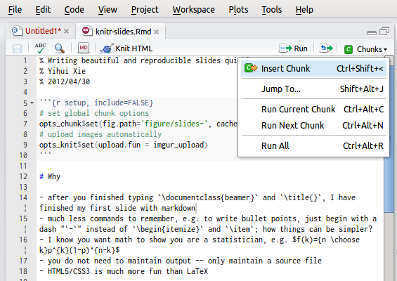
One week ago I made an early announcement about the markdown support in the knitr package and RStudio, and now the version 0.5 of knitr is on CRAN, so I’m back to show you how I made the HTML5 slides. For those who are not familiar with markdown, you may read the traditional documentation, but RStudio has a quicker reference (see below). The problem with markdown is that the original invention seems to be too simple, so quite a few variants were derived later (e.g. to support tables); that is another story, and you do not need to worry much about it.
Before you get started, make sure your knitr version is at least 0.5:
# install.packages(c('knitr', 'XML', 'RCurl'))
update.packages(ask = FALSE)
packageVersion('knitr') >= 0.5
Editor: RStudio
You need to install the RStudio preview version to use its new features on markdown support. With this version, you will see an interface like this when you create an R markdown file (File --> New --> R Markdown):

The button MD in the toolbar shows a quick reference of the markdown syntax, which I believe you can learn in 3 minutes. To start with, you can use my example on GitHub: knitr-slides.Rmd, or quickly cook up your own by Ctrl + Shift + I to insert code chunks.
You can write headers with # and bullet points with -. It is both quick to write and easy to remember (and readable too). When you are done, just hit the button Knit HTML, and you get a nice HTML page showing you R code and the output. You do not have to learn LaTeX in order to step into the realm of reproducible research. (Did you see the Binomial pmf there?!)
Converter: Pandoc
What happens behind the scene is that RStudio calls knitr to compile the Rmd document to a markdown file (you can see it under the same directory as the Rmd file), and convert this file to HTML. This is a very nice feature, and we can actually go further.
Pandoc claims itself to be a universal document converter, and it is indeed very powerful. For the above example, we can convert the markdown output (not Rmd source) to many other formats like HTML, LaTeX, Open Office or Microsoft Office documents. HTML5 slides are also supported. This is the single command that I used to convert knitr-slides.md to DZslides:
pandoc -s -S -i -t dzslides --mathjax knitr-slides.md -o knitr-slides.html
Then you get an HTML file knitr-slides.html which you can view in a modern web browser. Enjoy.
Final words
HTML5 slides is just one tiny thing that you can play with markdown; check out the pandoc documentation to see more possibilities. That being said, I feel most excited about the RStudio integration with knitr and markdown. LaTeX is beautiful but difficult to learn and laborious to write. MS Word is most widely used but you know…
I believe this combination makes reproducible research much more accessible to the general audience, and I hope to see it being used in statistical courses so that students no longer do tedious jobs of copy & paste, and professors no longer suffer from ugly Word reports.
Now I have done pretty much what I planned in the beginning. The next step will be our GSoC project, in which we will make the toolchain smoother, and work out better ways for R users to document packages and publish web pages (e.g. blogging like a hacker). If you want to follow our latest changes, you may
- watch the development repository on GitHub https://github.com/yihui/knitr
- or join the Google mailing list https://groups.google.com/group/knitr
And final ads: I will be presenting knitr at useR! 2012 with JJ from RStudio. I’m looking forward to meeting more knitters in Nashville :)