Here are some (trivial) R tips in the course Stat 511. I’ll update this post till the semester is over.
Formatting R Code
Reading code is pain, but the well-formatted code might alleviate the pain a little bit. The function tidy_source() in the formatR package can help us format our R code automatically. By default it will read your code in the clipboard, parse it and return the well-formatted code. You have options to keep or remove the comments/blank lines and set the width of the code, etc. Spaces and indent will be added automatically. This can save us time typing spaces and paying attention to indent.
## install.packages('formatR') if it is not installed yet
library(formatR)
## copy some R code somewhere and type:
tidy_source()
## or specify the path of your code file
tidy_source(system.file("demo", "image.R", package = "graphics"))
## can also use a URL
tidy_source('http://www.public.iastate.edu/~dnett/S511/twofactor.R')
## remove blank lines
tidy_source('http://www.public.iastate.edu/~dnett/S511/twofactor.R',
           keep.blank.line = FALSE)
## remove comments
tidy_source('http://www.public.iastate.edu/~dnett/S511/twofactor.R',
           keep.comment = FALSE)
Approximating Rationals by Fractions
We often deal with matrices like \(C(X'X)^{-1}X'\) in 511 and may wonder what on earth they are. If we directly compute solve(t(X) %*% X) %*% t(X) (or generalized inverse ginv() in MASS) we often end up with seeing a lot of decimals, which makes it difficult to see what these numbers really mean. The function fractions() in the MASS package can approximate rationals by fractions. For example:
## from the movie rating example
X = matrix(c(1, 1, 0, 0, 0, 1, 0, 0, 1, 1, 0, 0, 0,
    0, 1, 0, 1, 0, 1, 0, 0, 0, 1, 0, 1, 0, 1, 0, 0, 0, 0, 1,
    1, 0, 0, 1, 0, 0, 0, 1, 1, 0, 0, 0, 1, 1, 0, 0, 1, 0, 0,
    0, 1, 0, 1, 0), byrow = T, nrow = 7)
XX = t(X) %*% X
library(MASS)
XXgi = ginv(XX)
C = matrix(c(1, 1, 0, 0, 0, 1, 0, 0, 1, 1, 0, 0, 0,
    0, 1, 0, 1, 1, 0, 0, 0, 0, 0, 1, 1, 0, 1, 0, 0, 1, 0, 0,
    1, 0, 1, 0, 0, 0, 1, 0, 1, 0, 1, 0, 0, 0, 0, 1, 1, 0, 0,
    1, 0, 1, 0, 0, 1, 0, 0, 1, 0, 0, 1, 0, 1, 0, 0, 1, 0, 0,
    0, 1, 1, 0, 0, 0, 1, 1, 0, 0, 1, 0, 0, 0, 1, 0, 1, 0, 1,
    0, 0, 0, 1, 0, 0, 1), byrow = T, nrow = 12)
## what does C(X'X)^{-}X' mean?
#   hard to see
C %*% XXgi %*% t(X)
#               [,1]          [,2]          [,3]          [,4]
# [1,]  7.500000e-01  2.500000e-01  2.220446e-16  5.551115e-17
# [2,]  2.500000e-01  7.500000e-01  1.387779e-16  5.551115e-17
# [3,]  2.500000e-01  7.500000e-01 -1.000000e+00  1.000000e+00
# [4,]  5.000000e-01 -5.000000e-01  1.000000e+00  0.000000e+00
# [5,] -1.665335e-16 -5.551115e-17  1.000000e+00 -2.220446e-16
# [6,]  3.330669e-16  1.110223e-16  1.110223e-16  1.000000e+00
# [7,]  5.000000e-01 -5.000000e-01  1.000000e+00 -1.000000e+00
# [8,] -5.551115e-16 -3.330669e-16  1.000000e+00 -1.000000e+00
# [9,] -5.551115e-17 -2.220446e-16 -1.665335e-16  1.110223e-16
#[10,]  2.500000e-01 -2.500000e-01 -1.110223e-16  3.053113e-16
#[11,] -2.500000e-01  2.500000e-01 -2.220446e-16  2.775558e-16
#[12,] -2.500000e-01  2.500000e-01 -1.000000e+00  1.000000e+00
#               [,5]          [,6]          [,7]
# [1,]  2.775558e-17  2.500000e-01 -2.500000e-01
# [2,] -1.665335e-16 -2.500000e-01  2.500000e-01
# [3,] -4.440892e-16 -2.500000e-01  2.500000e-01
# [4,]  4.440892e-16  5.000000e-01 -5.000000e-01
# [5,]  2.220446e-16  0.000000e+00  1.110223e-16
# [6,]  1.110223e-16  0.000000e+00 -2.220446e-16
# [7,]  1.000000e+00  5.000000e-01 -5.000000e-01
# [8,]  1.000000e+00  2.220446e-16  4.440892e-16
# [9,]  1.000000e+00  2.775558e-16  1.110223e-16
#[10,] -5.551115e-17  7.500000e-01  2.500000e-01
#[11,] -2.220446e-16  2.500000e-01  7.500000e-01
#[12,] -6.661338e-16  2.500000e-01  7.500000e-01

#   much easier using fractions
fractions(C %*% XXgi %*% t(X))
#      [,1] [,2] [,3] [,4] [,5] [,6] [,7]
# [1,]  3/4  1/4    0    0    0  1/4 -1/4
# [2,]  1/4  3/4    0    0    0 -1/4  1/4
# [3,]  1/4  3/4   -1    1    0 -1/4  1/4
# [4,]  1/2 -1/2    1    0    0  1/2 -1/2
# [5,]    0    0    1    0    0    0    0
# [6,]    0    0    0    1    0    0    0
# [7,]  1/2 -1/2    1   -1    1  1/2 -1/2
# [8,]    0    0    1   -1    1    0    0
# [9,]    0    0    0    0    1    0    0
#[10,]  1/4 -1/4    0    0    0  3/4  1/4
#[11,] -1/4  1/4    0    0    0  1/4  3/4
#[12,] -1/4  1/4   -1    1    0  1/4  3/4
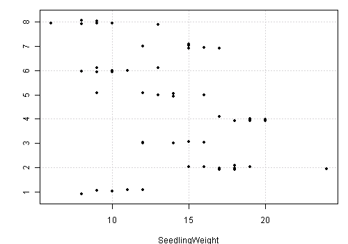
Jittered Strip Chart
Strip chart is a common tool for batch comparisons. When points get overlapped in the plot, we may “jitter” the points by adding a little noise to the data. The R function jitter() is an option to manipulate the data, but stripchart() already supports jittered points.
## some people do not realize that the 'colClasses' argument in
# read.table() is quite useful -- can avoid explicit conversion
d = read.table("http://dnett.public.iastate.edu/S511/SeedlingDryWeight2.txt",
header = TRUE, colClasses = c("factor", "factor", "factor",
"numeric"))
## R base graphics: method = 'jitter' will do
stripchart(SeedlingWeight ~ Tray, data = d, method = "jitter",
pch = 20, panel.first = grid())
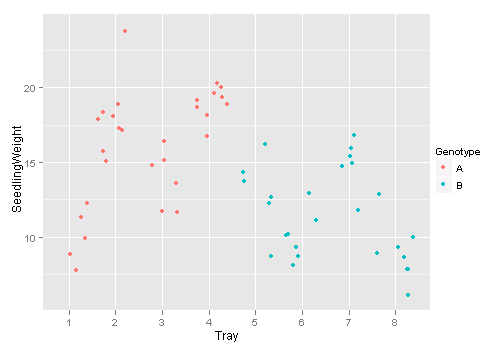
## or the ggplot2 version: geom = 'jitter'
library(ggplot2)
qplot(Tray, SeedlingWeight, data = d, colour = Genotype, geom = "jitter")
Testing \(C \beta = d\) in a Linear Model
R base does not provide a general test for the coefficients of a linear model, but we can use the function glh.test() in the gmodels package to do it. If you take a look at its source code, you will find unsurprisingly it is nothing but the code in page 7 of slide set 9 of Dr Nettleton’s lecture notes.
library(gmodels)
time = factor(rep(c(3, 6), each = 5))
temp = factor(rep(c(20, 30, 20, 30), c(2, 3, 4, 1)))
y = c(2, 5, 9, 12, 15, 6, 6, 7, 7, 16)
d = data.frame(time, temp, y)
o = lm(y ~ time + temp + time:temp, data = d)

## compare with page 7-11 in slide set 9

Ctime = matrix(c(0, 1, 0, 0.5), nrow = 1, byrow = T)
glh.test(o, Ctime)

#           Test of General Linear Hypothesis
#  Call:
#  glh.test(reg = o, cm = Ctime)
#  F = 6.0051, df1 = 1, df2 = 6, p-value = 0.04975

Ctemp = matrix(c(0, 0, 1, 0.5), nrow = 1, byrow = T)
glh.test(o, Ctemp)

#           Test of General Linear Hypothesis
#  Call:
#  glh.test(reg = o, cm = Ctemp)
#  F = 39.7072, df1 = 1, df2 = 6, p-value = 0.0007447

Ctimetempint = matrix(c(0, 0, 0, 1), nrow = 1, byrow = T)
glh.test(o, Ctimetempint)

#           Test of General Linear Hypothesis
#  Call:
#  glh.test(reg = o, cm = Ctimetempint)
#  F = 0.1226, df1 = 1, df2 = 6, p-value = 0.7382

Coverall = matrix(c(0, 1, 0, 0, 0, 0, 1, 0, 0, 0,
 0, 1), nrow = 3, byrow = T)
glh.test(o, Coverall)

#           Test of General Linear Hypothesis
#  Call:
#  glh.test(reg = o, cm = Coverall)
#  F = 13.5319, df1 = 3, df2 = 6, p-value = 0.004439
Demo for the F Distribution
I created a dynamic demo to illustrate the power of the F test here: Demonstrating the Power of F Test with gWidgets. Play with it and have fun!
Tricks in read.table()
Many people do not realize the possibility of converting the data types of columns in read.table() and always use such specific post hoc conversion:
soup = read.table("http://www.public.iastate.edu/~dnett/S511/soup.txt",
    header = TRUE)
soup$taster = factor(soup$taster)
soup$batch = factor(soup$batch)
soup$recipe = factor(soup$recipe)
soup$tasteorder = factor(soup$tasteorder)
But in fact, we can specify the types of columns while reading data:
## we know the first 4 are factors and the last one is numeric:
soup = read.table("http://www.public.iastate.edu/~dnett/S511/soup.txt",
    TRUE, colClasses = c(rep("factor", 4), "numeric"))
## conversion already done!
str(soup)
# 'data.frame':   72 obs. of  5 variables:
#  $ recipe    : Factor w/ 4 levels "1","2","3","4": 1 1 1 1 1 1 2 2 2 2 ...
#  $ batch     : Factor w/ 12 levels "1","10","11",..: 1 1 1 1 1 1 5 5 5 5 ...
#  $ taster    : Factor w/ 24 levels "1","10","11",..: 1 12 18 19 20 21 1 12 18 19 ...
#  $ tasteorder: Factor w/ 3 levels "1","2","3": 1 1 2 2 3 3 2 3 1 3 ...
#  $ y         : num  3 5 6 4 4 3 6 9 6 7 ...
There are other tips in read.table() but I find this one the most useful. Check the 22 arguments in ?read.table if you want to know more magic (e.g. how to specify the first column in the data file as the row names).
Demo for Newton’s Method
There is a function newton.method() in the package animation which shows the detailed iterations in Newton’s method. Here is a demo:
library(animation)
par(pch = 20)
ani.options(nmax = 50)
newton.method(function(x) 5 * x^3 - 7 * x^2 - 40 *
    x + 100, 7.15, c(-6.2, 7.1))
I hope this is useful for understanding iterative algorithms.
Misc Tips
Some more tips:
-
unname(): to remove the names of objectsx = c(a = 1, b = 2) x # a b # 1 2 unname(x) ## x = unname(x) if one wants to replace x # [1] 1 2
Donate
As a freelancer (currently working as a contractor) and a dad of three kids, I truly appreciate your donation to support my writing and open-source software development! Your contribution helps me cope with financial uncertainty better, so I can spend more time on producing high-quality content and software. You can make a donation through methods below.
-
Venmo:
@yihui_xie, or Zelle:[email protected] -
Paypal
-
If you have a Paypal account, you can follow the link https://paypal.me/YihuiXie or find me on Paypal via my email
[email protected]. Please choose the payment type as “Family and Friends” (instead of “Goods and Services”) to avoid extra fees. -
If you don’t have Paypal, you may donate through this link via your debit or credit card. Paypal will charge a fee on my side.
-
-
Other ways:
WeChat Pay (微信支付:谢益辉) Alipay (支付宝:谢益辉) 

When sending money, please be sure to add a note “gift” or “donation” if possible, so it won’t be treated as my taxable income but a genuine gift. Needless to say, donation is completely voluntary and I appreciate any amount you can give.
Please feel free to email me if you prefer a different way to give. Thank you very much!
I’ll give back a significant portion of the donations to the open-source community and charities. For the record, I received about $30,000 in total (before tax) in 2024-25, and gave back about $15,000 (after tax).