The other day I sent a small assignment to a group of people in order that they could play with statistics and become more interested with this subject. The data-generating process was quite simple: first I generated 20000 random numbers (10000 rows, 2 columns) from N(0, 1) and then add 10000 rows of numbers which lie exactly on a circle; at last I provided this data in a randomized order so people cannot easily discover the pattern just from the numbers.
The question is, how to reveal the particular pattern in this “pile of sand”? Let’s look at the original plot:
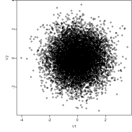
What can we observe from this scatter plot? Perhaps nothing but “a pile of sand”. However, if we choose alternative ways to create the plot again, things will be completely different. Here are my approaches:
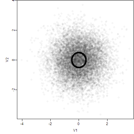
1. Use Semi-transparent Colors
Actually there are 10000 points lying on the circle, so the critical problem is overlapping. In order to show the degree of overlapping, we can use semi-transparent colors, because the color will be more opaque if there are many points at the same place.
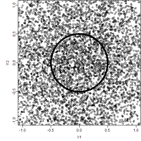
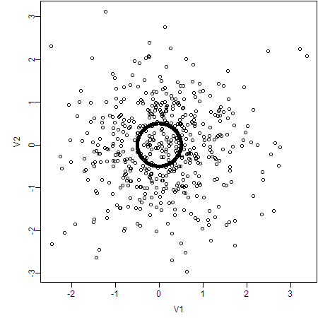
2. Set Axes Limits
If we look closer into the plot, the scene will also be different. For example, we only plot the data in the range [-1, 1].
3. Plot with Smaller Point Symbols
Certainly, small symbols can prevent overlapping effectively in this case.
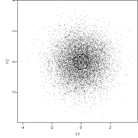
4. Draw A Subset of the Data
As the problem is that there are too many data points, why not draw a subset and try a scatter plot first? For example, here we have sampled 1000 rows of data and the plot is like this:
5. Estimate the 2D Density
The R package KernSmooth has provided functions to estimate the 1D or 2D density.We can further examine the shape of this 2D density using the package rgl. Here is an animation recorded to illustrate the 2D density.
The R code for the above plots & animation is as follows:
# generate the data
x = rbind(matrix(rnorm(10000 * 2), ncol = 2), local({
  r = runif(10000, 0, 2 * pi)
  0.5 * cbind(sin(r), cos(r))
}))
x = as.data.frame(x[sample(nrow(x)), ])

devAskNewPage(TRUE)
# original plot
plot(x)
# transparent colors (alpha = 0.1)
plot(x, col = rgb(0, 0, 0, 0.1))
# set axes lmits
plot(x, xlim = c(-1, 1), ylim = c(-1, 1))
# small symbols
plot(x, pch = ".")
# subset
plot(x[sample(nrow(x), 1000), ])

# 2D density estimation
library(KernSmooth)
fit = bkde2D(as.matrix(x), c(0.1, 0.1))
# perspective plot by persp()
persp(fit$x1, fit$x2, fit$fhat)

library(rgl)
# perspective plot by OpenGL
rgl.surface(fit$x1, fit$x2, 5 * fit$fhat)
# animation
M = par3d("userMatrix")
play3d(par3dinterp(userMatrix = list(M,
  rotate3d(M, pi/2, 1, 0, 0), rotate3d(M, pi/2, 0, 1, 0),
  rotate3d(M, pi, 0, 0, 1))), duration = 20)
Donate
As a freelancer (currently working as a contractor) and a dad of three kids, I truly appreciate your donation to support my writing and open-source software development! Your contribution helps me cope with financial uncertainty better, so I can spend more time on producing high-quality content and software. You can make a donation through methods below.
-
Venmo:
@yihui_xie, or Zelle:[email protected] -
Paypal
-
If you have a Paypal account, you can follow the link https://paypal.me/YihuiXie or find me on Paypal via my email
[email protected]. Please choose the payment type as “Family and Friends” (instead of “Goods and Services”) to avoid extra fees. -
If you don’t have Paypal, you may donate through this link via your debit or credit card. Paypal will charge a fee on my side.
-
-
Other ways:
WeChat Pay (微信支付:谢益辉) Alipay (支付宝:谢益辉) 

When sending money, please be sure to add a note “gift” or “donation” if possible, so it won’t be treated as my taxable income but a genuine gift. Needless to say, donation is completely voluntary and I appreciate any amount you can give.
Please feel free to email me if you prefer a different way to give. Thank you very much!
I’ll give back a significant portion of the donations to the open-source community and charities. For the record, I received about $30,000 in total (before tax) in 2024-25, and gave back about $15,000 (after tax).