The Graphics Manual
The graphics manual shows all cool bells and whistles about graphics in knitr.
- Source and output of the graphics manual
- Rnw source: knitr-graphics.Rnw
- LyX source: knitr-graphics.lyx
- PDF output: knitr-graphics.pdf
You will probably realize how much room there is for improvement of R graphics in publications. Don’t accept whatever R gives you; it is time starting making your graphics beautiful and professional.
A few screenshots from the manual:
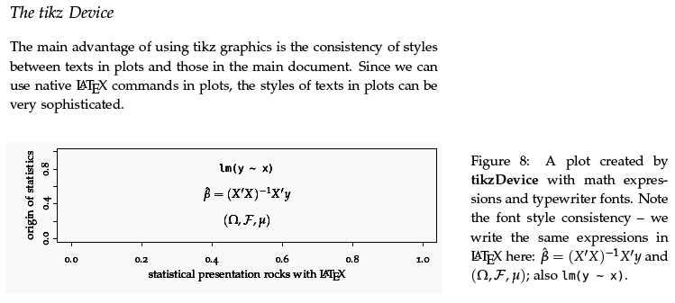
I’d like to thank the authors of the tufte-handout class, based on which this document was written, and the tikzDevice package makes the font styles in plots consistent with the document class (using serif fonts).
A note on custom graphical devices
The chunk option dev accepts custom graphical devices which can be defined as an R function with three arguments. Here is an example of a PDF device using pointsize 10:
<<custom-dev>>=
my_pdf = function(file, width, height) {
  pdf(file, width = width, height = height, pointsize = 10)
}
@
Then we can use this device in chunk options, but one important thing to remember is to provide the fig.ext option at the same time, because knitr is unable to guess what should be a correct file extension for the plot file. Finally we will use the custom device like this:
<<dev-demo, dev='my_pdf', fig.ext='pdf'>>=
plot(rnorm(100))
@
Of course you can set them globally using \SweaveOpts{} if you want to use this device through out the document.
Passing more arguments to a device
We can actually have even finer control over graphical devices through the dev.args option. Instead of hardcoding pointsize = 10, we can add an option dev.args = list(pointsize = 10) to the chunk. Here is an example:
<<pdf-pointsize, dev='pdf', dev.args=list(pointsize=10)>>=
plot(rnorm(100))
@
Since dev.args is a list, it can take any possible device arguments, e.g. dev.args=list(pointsize=11, family='serif') for the pdf() device. All elements of dev.args are passed to the graphical device of the chunk.
Create hyperlinks in R graphics
With the help of the tikzDevice package, we can write almost any LaTeX commands in R graphics. Here is an example links.Rnw of writing hyperlinks (courtesy of Jonathan Kennel).
An important note is you have to add \usepackage{hyperref} to the list of metrics packages used by tikzDevice, otherwise the command \hyperlink or \hypertarget will not be recognized.
Encoding of multibyte characters
When your plots contain multibyte characters, you may need set the encoding option of the pdf() device; see #172 for a discussion. For a possible list of encodings, see
list.files(system.file('enc', package = 'grDevices'))
## e.g. you can set pdf.options(encoding = 'CP1250')
You probably need to set the encoding when you see a warning like this: Warning: conversion failure on '<var>' in 'mbcsToSbcs': dot substituted for <var>.
Another possibility is to use the cairo_pdf device instead of pdf (see #436):
options(device = function(file, width = 7, height = 7, ...) {
  cairo_pdf(tempfile(), width = width, height = height, ...)
})
If that fails under Windows, you may also take a look at #527.
The Dingbats font
According to the documentation of pdf(), the useDingbats argument can reduce the file size of PDF’s which contain small circles. If you are using knitr in RStudio, this option is disabled by default. You may want to enable it by putting pdf.options(useDingbats = TRUE) in your source document if you have large scatter plots. See #311 for more comments and discussions.
Animations
When the chunk option fig.show='animate' and there are multiple plots produced from a code chunk, all plots will be combined to an animation. For LaTeX output, the LaTeX package animate is used to create animations in PDF. For HTML/Markdown output, by default FFmpeg is used to create a WebM video. Note you have to enable the libvpx support when installing FFmpeg. Linux and Windows users can just follow the download links on the FFmpeg website (libvpx has been enabled in the binaries). For OS X users, you can install FFmpeg via Homebrew
brew install ffmpeg --with-libvpx
Donate
As a freelancer (currently working as a contractor) and a dad of three kids, I truly appreciate your donation to support my writing and open-source software development! Your contribution helps me cope with financial uncertainty better, so I can spend more time on producing high-quality content and software. You can make a donation through methods below.
-
Venmo:
@yihui_xie, or Zelle:[email protected] -
Paypal
-
If you have a Paypal account, you can follow the link https://paypal.me/YihuiXie or find me on Paypal via my email
[email protected]. Please choose the payment type as “Family and Friends” (instead of “Goods and Services”) to avoid extra fees. -
If you don’t have Paypal, you may donate through this link via your debit or credit card. Paypal will charge a fee on my side.
-
-
Other ways:
WeChat Pay (微信支付:谢益辉) Alipay (支付宝:谢益辉) 

When sending money, please be sure to add a note “gift” or “donation” if possible, so it won’t be treated as my taxable income but a genuine gift. Needless to say, donation is completely voluntary and I appreciate any amount you can give.
Please feel free to email me if you prefer a different way to give. Thank you very much!
I’ll give back a significant portion of the donations to the open-source community and charities. For the record, I received about $30,000 in total (before tax) in 2024-25, and gave back about $15,000 (after tax).